Inflation and Recession

With the fear of recession rising, market participants have begun to reposition. Specifically, since June 14^th, we’ve seen falling interest rates as the 10-year treasury dropped 16.38%, oil dropped 15.19%, and equities have found some footing jumping 3.2%. However, these market moves are designed around the changing landscape that slower economic activity will (1) produce a mild recession, (2) bring down inflation, and (3) stop the Fed hiking cycle. In this article, I want to evaluate whether (1) is the inflationary gap narrowing (aka returning to trend) or are we falling into a recessionary gap, and (2) address how recessions impact inflation.

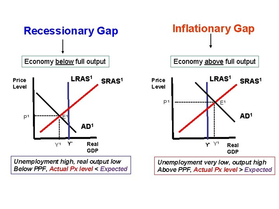
To begin, I believe it will help the reader if they understand the difference between a recessionary gap and an inflationary gap. The basis for these gaps starts with employment. Specifically, if the current unemployment rate is higher than the trend rate of unemployment, then the economy is producing less than is optimal. Fewer workers can cause GDP to drop below trend creating a recessionary gap. However, if the unemployment rate is below the trend rate of unemployment and the economy is producing at a theoretical full employment capacity, then GDP can drift above trend, creating an inflationary gap capable of producing inflation.

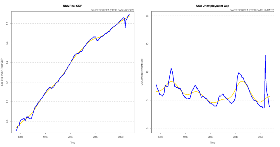
Visually, as seen in Figure 1, you can see that the economy is currently in an inflationary gap as the unemployment rate is well below the trend rate of unemployment and GDP runs above its 1976 trend.

British economist John Hicks combined these concepts to create his theory of the GDP Trade Cycle. Specifically, Hicks theorized that output had an upper and lower barrier. The upper barrier is determined by full employment, while the lower barrier is defined by the fact that net investment cannot fall below a certain negative level since gross investment cannot be less than zero, given depreciation warrants equipment repair/replacement (Kandor, 1951). Below I illustrate Hick’s model mathematically

Y=A+(1-s+v)*Y(t-1) - v*Y(t-2)

Where GDP (Y) is equal to autonomous GDP(A) plus the two previous periods of GDP affected by the marginal propensity to save (s) and (v) an investment coefficient (Sanderson, 2016). Hicks has already told us the upper boundary to the cycle is full employment. However, we must use this equation to estimate the lower boundary of the cycle or investment(v) in our equation above. We can do this by running a simple linear regression. The results are shown in Figure 2.

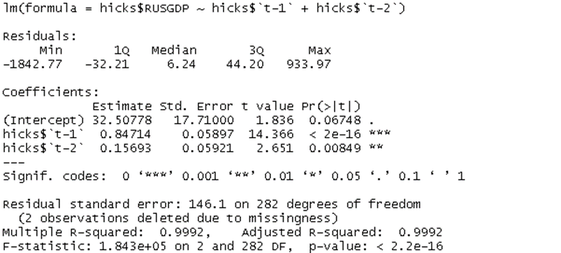
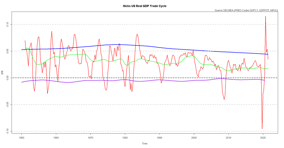
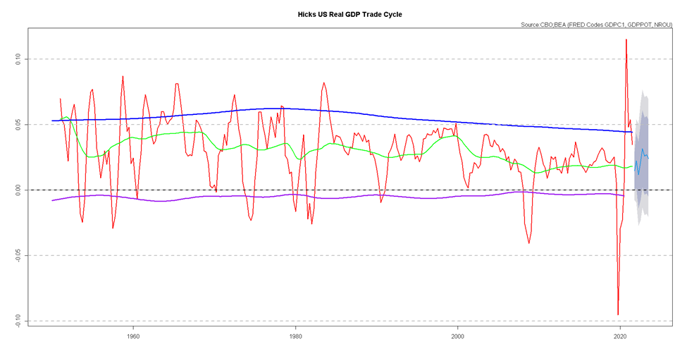
As you can see from the regression analysis, the coefficient on GDP lagged two periods, or (v) in the Hicks accelerator equation above, is 0.15693, suggesting that -0.15693*GDP could be the cycle floor. Putting Hicks’s Trade Cycle together, we get Figure 3 below, which reconfirms the inflationary gap from Figure 1 as Real GDP (shown in red) is above both the potential trend (shown in green) and Hicks’s upper barrier of full employment (shown in blue).

However, the recent demand destruction brought on by the rise in interest rates and tightening of financial conditions has reduced GDP over the last few quarters to the point where we must ask, are we simply returning to trend, or will we test Hicks’ lower barrier resulting in a recessionary gap? Figure 4 below highlights our current estimate of the year-over-year rate of change of real GDP for the next eight quarters suggesting this growth slowdown will likely return to trend.

This should intuitively make sense, given we have not yet seen job losses during this cycle. Figure 5 below highlights the change in unemployment during a recession. On average, the unemployment rate rises by 3.2% during a recession of about ten months. When we look at the periods with CPI above 8.0% (’73-’75, ’80-’82), the unemployment rate starts at around 5.60% and increases to 4.10% by the recession’s end. These stats suggest that the unemployment rate must rise substantially from here for us to claim a deeper recession or that GDP will fall to Hicks’s lower barrier. I will say that this outcome is possible as the 95% confidence band (shown in grey) in Figure 4 does bring Hick’s lower barrier into play. However, you likely need the unemployment rate to rise above trend quickly for this to happen.

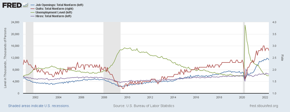
With that in mind, we must determine if the unemployment rate is about to rise. We have seen initial claims increase from the lows of March, 166k claims, to today’s 233K weekly filings. Despite this rise in claims, the most recent JOLTS report suggests there are still a record number of job openings (11.24 million) compared to those unemployed (5.95 million). Though, total hires are more in line with the unemployed at 6.489 million, suggesting (1) that although there are positions opened, many firms are allowing those jobs to go unfilled potentially due to rising input costs from the inflationary gap the economy is experiencing or (2) companies are having trouble attracting qualified candidates. I tend to believe the first story, but both can be true, as recent PMI survey data highlights the struggles of finding workers.

So, given employment is rising but not yet above trend, our base case must be that growth will return to trend. We must now ask if the decline in the economy will be enough to bring inflation back to the Fed’s 2% target. History finds this unlikely. As you can see in Figure 7, the average decline in Inflation during recessionary periods is -1.7%, suggesting a shorter temporary decline would not be enough to tame inflation. However, a more prolonged recession (such as the ’81-’82, and ’08-’09) saw significant reductions (-6.3%, -5.5%) in the inflation rate. Since our base case is a return to trend and not a recessionary gap, we see inflation remaining elevated by year-end, leaving room for the Fed to continue its tightening cycle despite the market’s optimism of a Powell pause or pivot. This will continue to produce less accommodative financial conditions that will pressure financial markets until inflation has materially moved lower.

The alternative case is we begin to see an accelerated pace of job losses which throws the economy into a recessionary gap. To see if this occurs, we must watch employment and private investments closely. Simplistically, the unemployment picture would be our first signal. Given that unemployment is the last shoe to drop in the cycle, it makes sense for this to begin rising. I’ve already mentioned this but a rapid rise in unemployment would take Hicks’s lower barrier from possible to probable.

Figure 8 highlights a second indicator to watch for this alternative case. The ratio of real gross private domestic investment to real gross domestic income. This indicator is lagging as investments tick up during and at the end of a recession. Hicks mentioned in his paper that there is always a level of autonomous investment given that equipment and structures will need to be repaired or replaced from depreciation. This implies that investments should remain stable during expansionary times and accelerate during recessionary times as the return on those investments would be more significant during recessionary times. As you can see from the chart below, whenever the ratio rises above 18.11, a large allocation of resources has been invested to create a catalyst for the beginning of the next economic cycle.

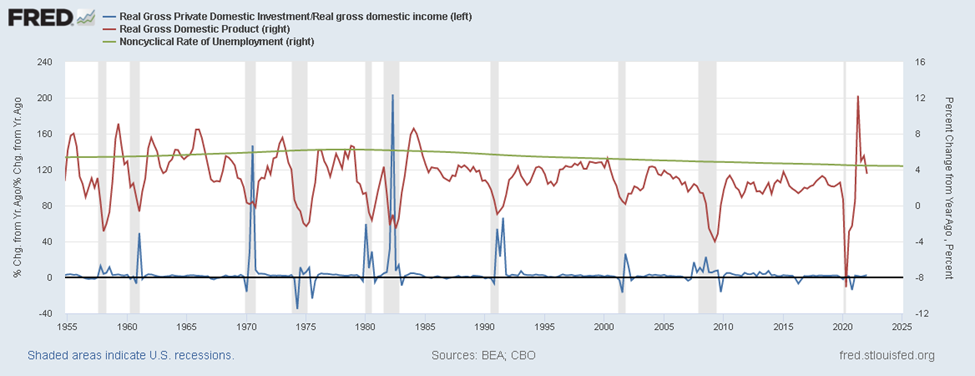
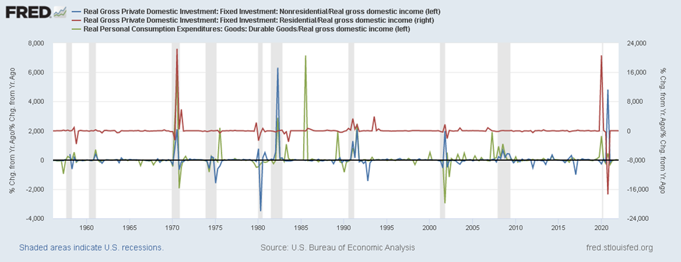
Figure 9 below shows the different components of real gross private domestic investments, highlighting that these investments must come from Nonresidential, Residential, or Consumer Durable Goods. However, all three investment components accelerated substantially post-covid, which I believe created a new cycle after the lockdowns. Therefore, if we fall into a recessionary gap, it will likely mean this cycle was significantly shorter than previous expansions meaning the investments made post covid were not enough to sustain a typical recovery. Finally, if this is a shorter cycle and job losses accelerate, the economy will need another boost of private investment to start the next economic cycle.

Sources

Kaldor, N. (1951). Mr. Hicks on the Trade Cycle. The Economic Journal, 61(244), 833–847. https://doi.org/10.2307/2226984

Sanderson, R. (2016). The Measurement of Economic Stability Over Time.

Hicks, John. A contribution to the Theory of the Trade Cycle. Clarendon Pr., 1950.